Jacobian
6R로봇의 경우 액추에이터에 가해진 토크로 Joint가 회전하게 되는데, 이로인해 링크가 움직이게 된다.
링크의 선속도와 각속도는 조인트 속도와 Jacobian 행렬을 통해 연결되며, 이는 로봇의 기구학적 관계를 나타낸다.
즉, Jacobian을 통해 미소 변위에서 비선형 변환을 선형 변환으로 근사시킬 수 있다.
따라서 Joint 좌표계에서 Cartesian 좌표계로 변환하기 위해서 Jacobian은 필수불가결한 내용이다. 그 역도 마찬가지다.
엔드 이펙터 컨피규레이션이 최소 좌표 집합(a minimal set of coordinates) x로 표현되고 속도 또한 $\dot x$로 표현되는 경우에, 정기구학 x(t)는 다음과 같이 표현할 수 있다.
$$x \in \mathbb{R}^m, \quad \dot{x} = \frac{dx}{dt} \in \mathbb{R}^m, \quad x(t) = f(\theta(t)), \quad \theta \in \mathbb{R}^n$$
θ는 관절 변수(각도)를 의미하며, 정기구학 x(t)를 시간에 대해 미분한 후 chain rule을 적용시키면
$\dot{x} = \frac{\partial f(\theta)}{\partial \theta} \frac{d\theta(t)}{dt} = \frac{\partial f(\theta)}{\partial \theta} \dot{\theta} = J(\theta) \dot{\theta}$
$ J(\theta) \in \mathbb{R}^{m \times n} $ J(θ)는 자코비안을 뜻하며, 자코비안 행렬은 관절 변위 θ에 대한 함수로써 관절속도 dθ/dt 에 대한 엔드 이펙터 속도 dx/dt의 기울기를 의미한다.
Example : 2R 평면 개연쇄 매니퓰레이터
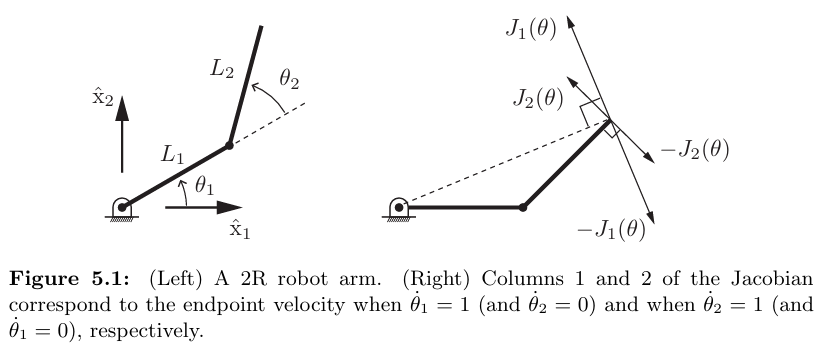
좌표 변환)
$x_1 = L_1 \cos\theta_1 + L_2 \cos(\theta_1 + \theta_2), \quad
x_2 = L_1 \sin\theta_1 + L_2 \sin(\theta_1 + \theta_2)$
속도 변환)
$\dot{x}_1 = -L_1 \dot{\theta}_1 \sin\theta_1 - L_2 (\dot{\theta}_1 + \dot{\theta}_2) \sin(\theta_1 + \theta_2), \quad
\dot{x}_2 = L_1 \dot{\theta}_1 \cos\theta_1 + L_2 (\dot{\theta}_1 + \dot{\theta}_2) \cos(\theta_1 + \theta_2)$
$\dot x = J(θ) \dot θ$ 꼴로 정리하면,
$$\begin{bmatrix}
\dot{x}_1 \\ \dot{x}_2
\end{bmatrix} =
\begin{bmatrix}
- L_1 \sin\theta_1 - L_2 \sin(\theta_1 + \theta_2) & - L_2 \sin(\theta_1 + \theta_2) \\
L_1 \cos\theta_1 + L_2 \cos(\theta_1 + \theta_2) & L_2 \cos(\theta_1 + \theta_2)
\end{bmatrix}
\begin{bmatrix}
\dot{\theta}_1 \\ \dot{\theta}_2
\end{bmatrix}$$
J(θ)의 각 열을 J1(θ), J2(θ)라 하고, tip velocity를 v_tip이라 하면,
$$v_{\text{tip}} = J_1(\theta) \dot{\theta}_1 + J_2(\theta) \dot{\theta}_2$$
J1(θ), J2(θ)가 일직선 상에 위치하지 않는 경우, 적절한 dθ1/dt dθ2/dt 값을 통해 tip velocity는 임의의 모든 방향을 나타낼 수 있다.
J1(θ), J2(θ)가 일직선 상에 위치하는 경우 자코비안 행렬 J(θ)는 특이 행렬이 되며, 이러한 컨피규레이션을 특이점(singularities)라 부르고, 이 경우 특정 방향을 향해 tip을 움직일 수 없다.
관절 속도 공간을 손끝 속도 공간으로 대응시켜 주어진 자세가 특이점에 얼마나 가까운지 정량적으로 측정할 수 있다.
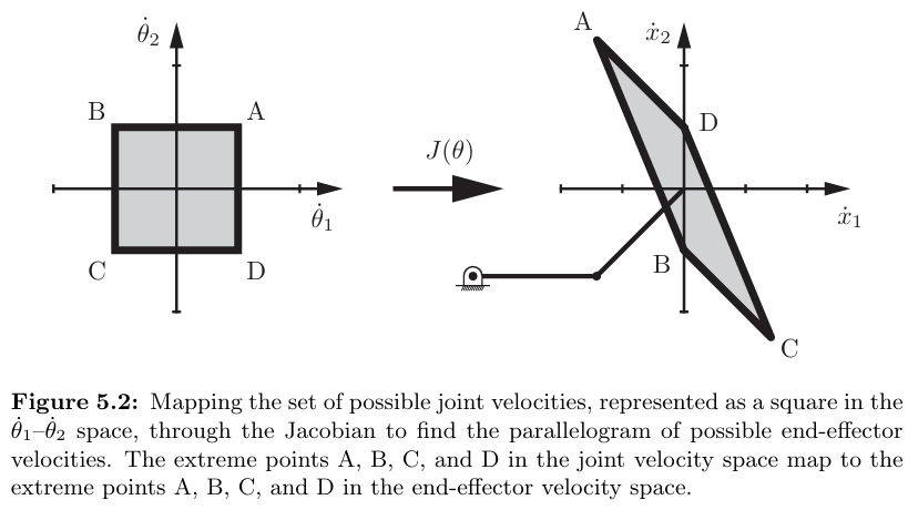
Figure 5.2의 경우 관절 속도 한곗값의 다각형을 자코비안을 통해 대응시키는 대신, 관절 속도 공간에서의 단위 원을 θ1 - θ2 평면으로 대응시키는 것도 가능하다.
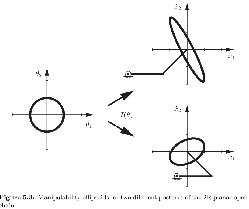
대응시켜 얻은 타원을 조작성 타원체라 부르며, 장축과 단측 비율이 1에 가까울수록 모든 방향으로 움직이기 쉬워지고 자세는 특이점으로부터 멀어진다. 반대로, 특이점에 가까워질수록 타원체는 선분에 가까워져 특정 방향으로 움직이지 못함을 나타낸다.
정역학에서도 비슷하게 자코비언을 통해 에너지와 힘을 분석할 수 있다.
Manipulatior Jacobian
$$\dot{x} = \frac{\partial f(\theta)}{\partial \theta} \frac{d\theta(t)}{dt} = \frac{\partial f(\theta)}{\partial \theta} \dot{\theta} = J(\theta) \dot{\theta}$$
손끝 속도와 관절 속도는 자코비언에 대해 선형적임을 알 수 있었다.
손끝 속도가 6차원 트위스트 V로 주어지는 경우,
- $V_s=J_s(\theta)\dot \theta$ 을 만족하는 공간 자코비언 $J_s(\theta)$
- $V_b= J_b(\theta)\dot\theta$을 만족하는 물체 자코비언 $J_b(\theta)$
으로 자코비안을 나타낼 수 있다.
공간 자코비안 $J_s(\theta)$
n 링크 개연쇄 정기구학을 지수 곱(PoE)으로 나타내면, $T(\theta_1, \dots, \theta_n) = e^{[S_1] \theta_1} e^{[S_2] \theta_2} \dots e^{[S_n] \theta_n} M$
공간 트위스트 V_s는 [V_s] = \dot T T^{-1 }으로 주어지며, \dot T 와 T^{-1} 는 다음과 같다.
$$\dot{T} = \left( \frac{d}{dt} e^{[S_1] \theta_1} \right) \cdots e^{[S_n] \theta_n} M
+ e^{[S_1] \theta_1} \left( \frac{d}{dt} e^{[S_2] \theta_2} \right) \cdots e^{[S_n] \theta_n} M + \dots$$
$$= [S_1] \dot{\theta}_1 e^{[S_1] \theta_1} \cdots e^{[S_n] \theta_n} M
+ e^{[S_1] \theta_1} [S_2] \dot{\theta}_2 e^{[S_2] \theta_2} \cdots e^{[S_n] \theta_n} M + \dots$$
$T^{-1} = M^{-1} e^{-[S_n] \theta_n} \cdots e^{-[S_1] \theta_1}$
대입하면,
$[V_s] = [S_1] \dot{\theta}_1 + e^{[S_1] \theta_1} [S_2] e^{-[S_1] \theta_1} \dot{\theta}_2
+ e^{[S_1] \theta_1} e^{[S_2] \theta_2} [S_3] e^{-[S_2] \theta_2} e^{-[S_1] \theta_1} \dot{\theta}_3 + \dots$
Adjoint mapping(수반 사상)을 이용하면 다음과 같이 정리할 수 있다.
$V_s = \underbrace{S_1}_{J_{s1}} \dot{\theta}_1
+ \underbrace{\text{Ad}_{e^{[S_1] \theta_1}} (S_2)}_{J_{s2}} \dot{\theta}_2
+ \underbrace{\text{Ad}_{e^{[S_1] \theta_1} e^{[S_2] \theta_2}} (S_3)}_{J_{s3}} \dot{\theta}_3 + \dots $
$V_s=J_s(\theta)\dot \theta$ 형태이므로,
$V_s = J_{s1} + J_{s2}(\theta) \dot{\theta}_1 + \dots + J_{sn}(\theta) \dot{\theta}_n$
행렬 형식으로 나타내면,
$V_s = \begin{bmatrix} J_{s1} & J_{s2}(\theta) & \dots & J_{sn}(\theta) \end{bmatrix}
\begin{bmatrix} \dot{\theta}_1 \\ \vdots \\ \dot{\theta}_n \end{bmatrix} = J_s(\theta) \dot{\theta}$
정리하면,
1. n 링크 개연쇄 정기구학을 지수 곱(PoE)으로 나타낼 수 있다.
$$T(\theta_1, \dots, \theta_n) = e^{[S_1] \theta_1} e^{[S_2] \theta_2} \dots e^{[S_n] \theta_n} M$$
2. 공간 자코비언 $J_s(\theta) \in \mathbb{R}^{6 \times n}$ 은 다음 식처럼 관절 속도 벡터 $\dot{\theta} \in \mathbb{R}^n$ 로부터 공간 트위스트를 구할 수 있다.
$$V_s=J_s(\theta)\dot \theta$$
3. $J_s(\theta)$의 $i$번째 열 ($i = 2, 3, \dots, n$)은 다음과 같다.
$$J_{si}(\theta) = \text{Ad}_{e^{[S_1] \theta_1} \dots e^{[S_{i-1}] \theta_{i-1}}} (S_i)$$
이때, 첫 번째 열은 $J_{s1}(\theta) = S_1$ 이다.
- $J_s(\theta)$ 의 물리적인 의미
각 열이 $Ad_{T_{i-1}}(S_i)$ 으로 주어짐을 생각해보면,
$T_{i-1} = \exp([S_1]\theta_1) \cdots \exp([S_{i-1}]\theta_{i-1})$이고, $S_i$는 영 위치에서 $i$번째 관절축이 공간 좌표계에서 표현된 것이다.
따라서 $Ad_{T_{i-1}}(S_i)$ 은 $i$ 번째 관절축이 $T_{i-1}$의 강체 운동으로 회전되는 것을 뜻한다.
이는 $i-1$개 관절을 각각 영 위치에서 현재 자세 $\theta_1, \cdots, \theta_{i-1}$ 로 움직이는 것과 같은 의미다.
다시 말하면, $J_s(\theta)$의 $i$번째 열 $J_{si}(\theta)$은 공간 좌표계에서 표현된 $i$번째 관절축을 관절 변위 $\theta_1, \cdots, \theta_{i-1}$ 에 대한 함수로 표현한 것이다.
물체 자코비안 $J_b(\theta)$
공간 자코비언과 비슷한 유도과정을 갖는다.
$\mathcal{V}_b = J_b(\theta) \dot{\theta}$
$J_{bi}(\theta) = \text{Ad}_{e^{-[B_n] \theta_n} \dots e^{-[B_{i+1}] \theta_{i+1}}} (B_i),$
$J_b(\theta)$의 각 열 $J_{bi}(\theta) = (\omega_{bi}(\theta), v_{bi}(\theta))$은 엔드 이펙터 좌표계에서 표현된 $i$번째 관절 축 스크류 벡터이다.
공간 자코비언과 다른 점은 $J_{bi}(\theta)$을 영 위치$(\theta = 0)$ 외 임의의 $\theta$에서 구하는 것이다.
공간 자코비언과 물체 자코비언의 관계식
공간 좌표계 $\{s\}$, 엔드 이펙터 좌표계 $\{b\}$, 정기구학 $T_{sb}(\theta)$ 라 하자.
엔드 이펙터 좌표계의 트위스트는 $\{s\}$, $\{b\}$ 각각에 대해
$$[\mathcal{V}_s] = \dot{T}_{sb} T_{sb}^{-1}, \quad
[\mathcal{V}_b] = T_{sb}^{-1} \dot{T}_{sb}$$
자코비안으로 나타내면,
$$\mathcal{V}_s = J_s(\theta) \dot{\theta}, \quad
\mathcal{V}_b = J_b(\theta) \dot{\theta}$$
$\mathcal{V}_s = \text{Ad}_{T_{sb}} (\mathcal{V}_b) \quad \text{and} \quad \mathcal{V}_b = \text{Ad}_{T_{bs}} (\mathcal{V}_s)$ 이므로,
$$\text{Ad}_{T_{sb}} (\mathcal{V}_b) = J_s(\theta) \dot{\theta}$$
양변에 $[Ad_{T_{bs}}]$ 을 곱하고 정리하면,
$$\text{Ad}_{T_{bs}} (\text{Ad}_{T_{sb}} (\mathcal{V}_b)) = \text{Ad}_{T_{bs} T_{sb}} (\mathcal{V}_b) = \mathcal{V}_b = \text{Ad}_{T_{bs}} (J_s(q) \dot{\theta})$$
모든 $\dot{\theta}$에 대해 $\mathcal{V}_b = J_b(\theta) \dot{\theta}$ 가 성립하므로,
$$J_b(\theta) = \text{Ad}_{T_{bs}} (J_s(\theta)) = [\text{Ad}_{T_{bs}}] J_s(\theta)$$
마찬가지로 공간 자코비안에 대해서도 유도하면,
$$J_s(\theta) = \text{Ad}_{T_{sb}} (J_b(\theta)) = [\text{Ad}_{T_{sb}}] J_b(\theta)$$
→ 공간 자코비언 - 물체 자코비언, 공간 트위스트 - 물체 트위스트 들 모두 수반 사상을 통해 변환된다.
이는 자코비언의 각 열이 트위스트에 해당하기 때문이다.
→ 공간 자코비언과 물체 자코비언은 항상 같은 rank을 갖는다.
Reference
1. Lynch, K. M., & Park, F. C. (2017). Modern robotics. Cambridge University Press.